Introduction
This blog post dives into the fascinating world of computer vision, exploring how we can teach machines to “see” using convolutional neural networks (CNNs). This post is based on a lecture from MIT’s 6.S191: Introduction to Deep Learning course.
What Does it Mean to “See”?
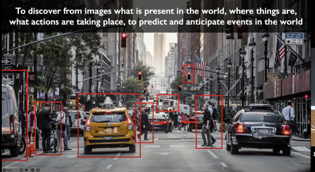
Before diving into the technical details, let’s define “vision”. It’s not simply about identifying objects in an image. True vision goes beyond object recognition to understand the relationships between objects, their movements, and their future trajectories. Think about how you intuitively anticipate a pedestrian crossing the street or a car changing lanes. Building machines with this level of visual understanding is the ultimate goal.
How Computers “See” Images
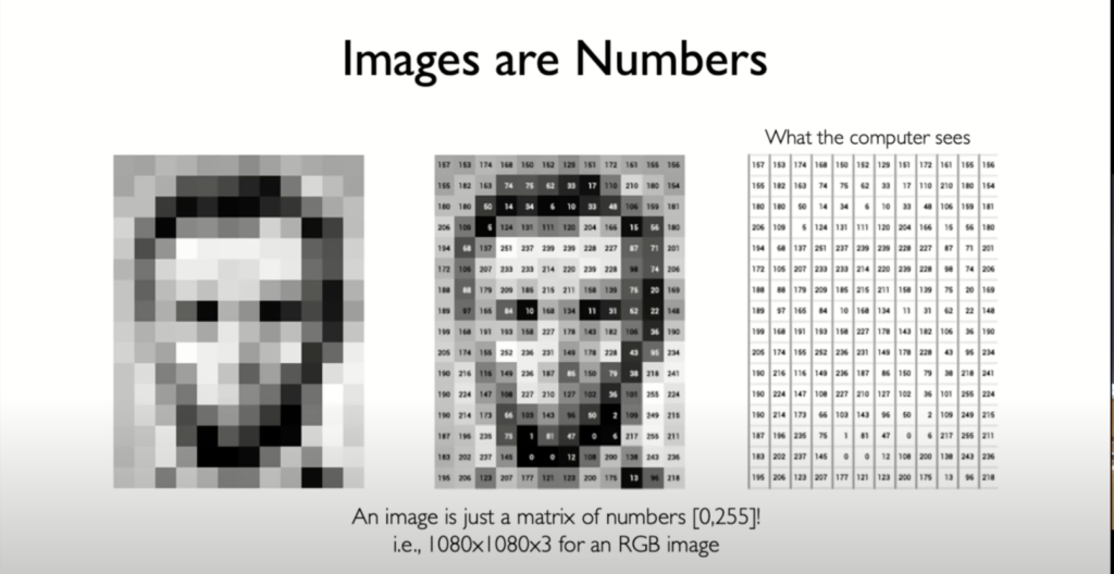
Unlike humans, computers perceive images as arrays of numbers, with each number representing the brightness level of a pixel. Grayscale images use a single number per pixel, while color images use three numbers (RGB) per pixel. Understanding this numerical representation is crucial for understanding how CNNs process visual information.
Let’s break down how an RGB image is represented as a three-dimensional array.
Grayscale Image Representation
First, let’s recap how a grayscale image is represented:
- A grayscale image consists of pixels, and each pixel represents a single value corresponding to its brightness or luminosity.
- This value can range from 0 (black) to 255 (white) in an 8-bit image.
- The image can be thought of as a two-dimensional array (or matrix), where each element in the array corresponds to the brightness value of a pixel.
- For example, a 100×100 pixel grayscale image can be represented as a 100×100 matrix.
RGB Image Representation
An RGB image is a bit more complex:
- An RGB image consists of pixels, and each pixel represents three color values: Red, Green, and Blue.
- Each of these color values can also range from 0 to 255 in an 8-bit image.
- Instead of a single brightness value per pixel (as in grayscale), an RGB pixel is represented by three values.
To represent this, we use a three-dimensional array:
- The first two dimensions correspond to the height and width of the image, just like in a grayscale image.
- The third dimension corresponds to the color channels (Red, Green, and Blue).
5×5 RGB Image Matrix
Let’s define some RGB values for illustration. Each inner list represents the RGB values of a pixel.
image = [
    # Row 0
    [[255, 0, 0], [0, 255, 0], [0, 0, 255], [255, 255, 0], [255, 0, 255]],
    # Row 1
    [[0, 255, 255], [128, 128, 128], [255, 128, 0], [0, 128, 255], [128, 0, 128]],
    # Row 2
    [[255, 255, 255], [0, 0, 0], [128, 255, 0], [255, 0, 128], [0, 255, 128]],
    # Row 3
    [[128, 0, 0], [0, 128, 0], [0, 0, 128], [128, 128, 0], [0, 128, 128]],
    # Row 4
    [[64, 64, 64], [192, 192, 192], [64, 192, 64], [192, 64, 192], [64, 64, 192]],
]
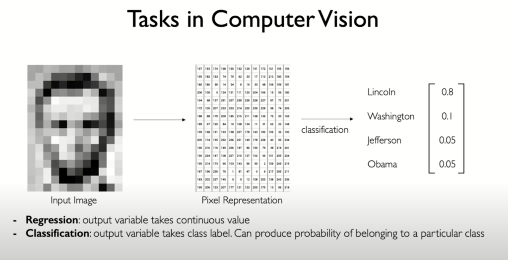
In the realm of computer vision, it’s crucial to understand two fundamental types of tasks: regression and classification.
Tasks in Computer Vision
- Regression: Outputs continuous values (e.g., predict the exact age of a person from a photograph. The output is a continuous value, like 25.7 years).
- Classification: Outputs discrete labels (e.g., identifying whether an image contains a cat or a dog).
Convolution Neural Netrworks
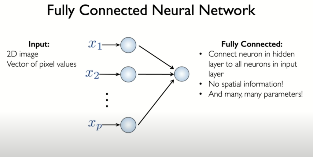
A fully connected neural network (FCNN) consists of multiple layers, including hidden layers, where each neuron in one layer is connected to every neuron in the previous and subsequent layers. When using an FCNN for image classification, we must flatten the 2D image into a 1D array, feeding each pixel into the network as an input. This approach has significant drawbacks:
- Loss of Geometric Structure: Flattening the image destroys the spatial relationships and local patterns inherent in the 2D structure. Important features related to pixel proximity are lost.
- Large Number of Parameters: Flattening a small 100×100 pixel image results in 10,000 input neurons. Connecting these to another layer with 10,000 neurons introduces 100 million parameters (10,000 x 10,000). This massive number of parameters is computationally inefficient and impractical for training and processing.
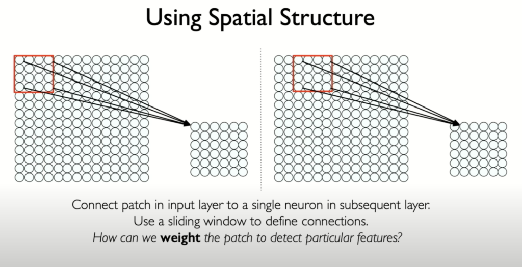
Instead of connecting every neuron to all pixels in the input image, we connect neurons in a hidden layer to small patches of the input image. This method maintains the spatial structure and reduces the number of parameters.
- Patch-Based Connections: Each neuron in the hidden layer is connected to a specific patch of pixels in the input image. For example, a red patch in the input image connects to a single neuron in the next layer. This neuron only sees a small part of the image, not the entire image.
- Correlation of Pixels: Pixels within a small patch are likely to be correlated, as they are close to each other. This property leverages the natural structure of images.
- Sliding Patches: To cover the entire image, the patch is slid across the input image, connecting patches to corresponding neurons in the hidden layer. This creates a new layer of neurons while preserving the spatial relationships from the input image.
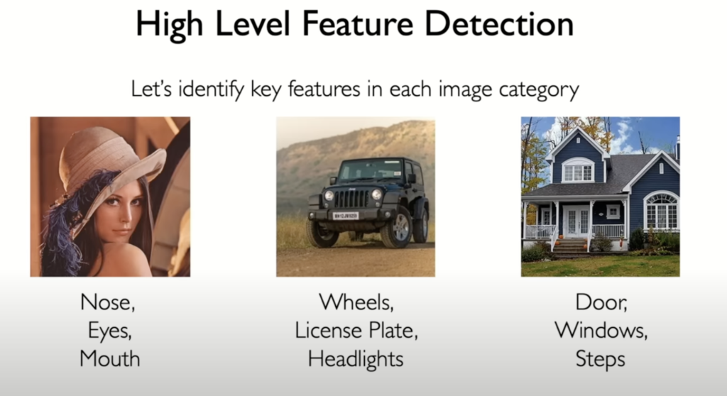
- Feature Detection: The ultimate goal is to detect visual patterns or features in the image. By connecting patches to hidden neurons and cleverly weighting these connections, neurons can specialize in detecting particular features within their patches.
This approach retains the spatial structure of the image and allows neurons to detect relevant features, making it more efficient and effective for image processing tasks compared to a fully connected network.
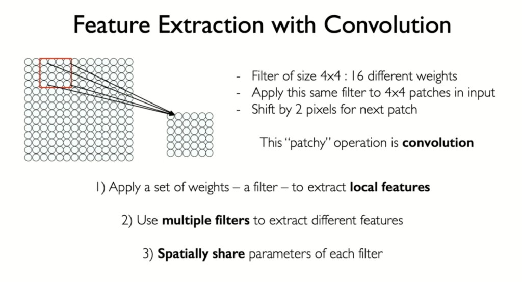
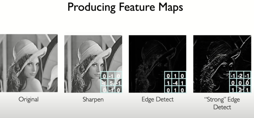
The Power of Convolution: Extracting Meaningful Features
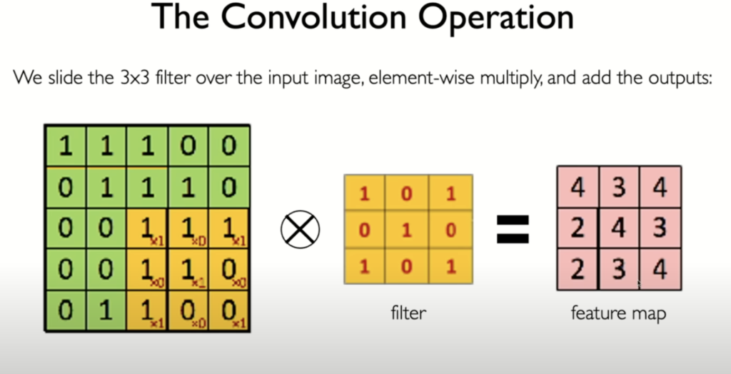
The heart of a CNN lies in its convolutional layers. These layers use filters (small matrices of weights) that slide across the image, performing element-wise multiplications and summations. This process creates feature maps, highlighting areas where the filter detects specific patterns.
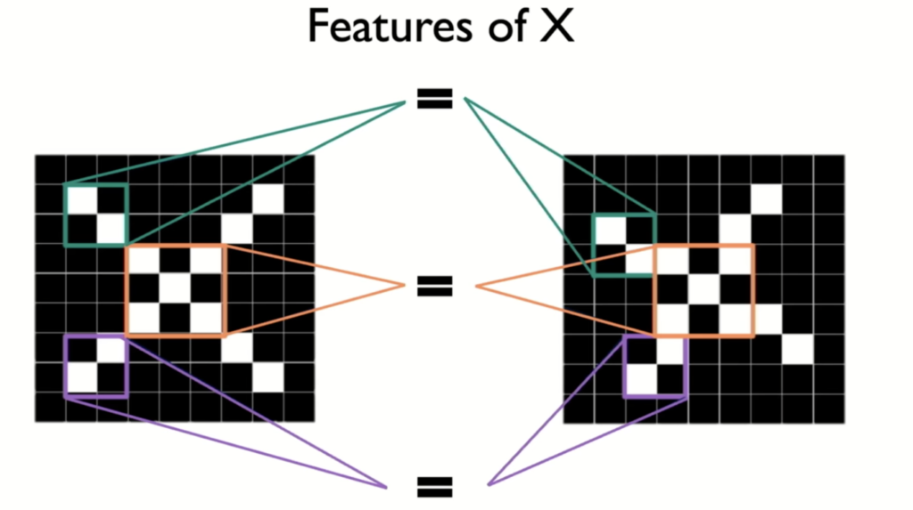
Let’s see a simple example of classifying “X” shapes to illustrate how different filters can detect different features within an image, such as diagonal lines and intersections, ultimately enabling the network to recognize the overall “X” shape.
Building Blocks of a CNN: Convolution, Non-linearity, and Pooling
Convolution in the context of convolutional neural networks (CNNs) is a mathematical operation used to extract features from input data, such as images, by applying a filter or kernel across the input. Here’s a detailed breakdown:
- Kernel/Filter: A small matrix (e.g., 3×3 or 5×5) with learnable parameters. The kernel slides over the input image to perform the convolution operation.
- Sliding/Striding: The kernel moves across the input image, typically from left to right and top to bottom. The step size of this movement is called the stride. For example, a stride of 1 means the kernel moves one pixel at a time, while a stride of 2 means it moves two pixels at a time.
- Convolution Operation: At each position, the kernel multiplies its values element-wise with the input pixels it overlaps, then sums these products to produce a single output value. This operation is repeated across the entire input image.
- Feature Map: The result of applying the convolution operation across the image is a feature map (or activation map), which highlights the presence of certain features detected by the kernel, such as edges, textures, or more complex patterns in deeper layers.
- Padding: Sometimes, the input image is padded with zeros around the border to control the spatial dimensions of the output feature map. Padding ensures that the kernel can process edge pixels and helps preserve the input dimensions.
- Non-linearity (ReLU): After convolution, a non-linear activation function, typically the Rectified Linear Unit (ReLU), is applied to introduce non-linearity into the model, enabling it to learn more complex patterns.
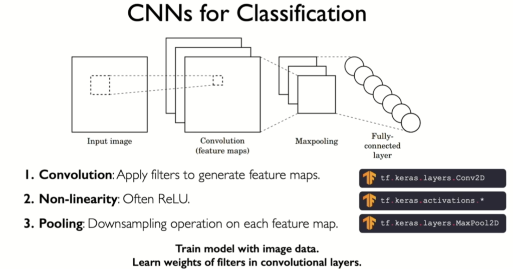
Beyond convolution, a typical CNN architecture incorporates two additional key elements:
- Non-linearity: After each convolution, a non-linear function (like ReLU) is applied to the feature map. This introduces non-linearity into the model, enabling it to learn more complex patterns.
- Pooling: This down-sampling operation reduces the dimensionality of the feature maps, making the network more computationally efficient and increasing the receptive field of subsequent layers.
In convolutional neural networks (CNNs), non-linearity and pooling operations are essential for enhancing feature extraction and reducing dimensionality.
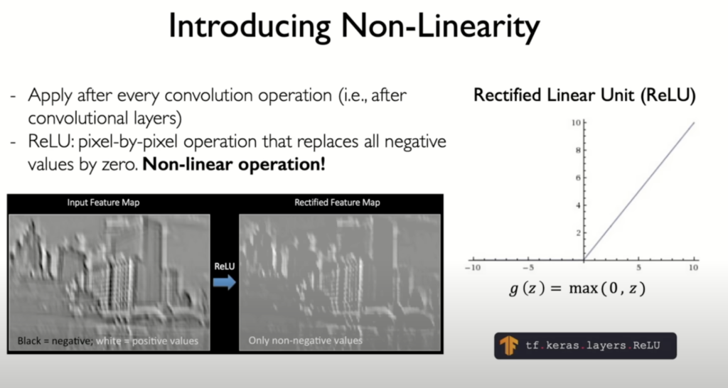
- Non-linearity:
- Purpose: Introduced because real-world data is highly nonlinear.
- Common Activation Function: Rectified Linear Unit (ReLU).
- Function: Deactivates negative values in the feature map by setting them to zero, while passing positive values unchanged. This acts like a threshold function, enhancing model capacity to learn complex patterns.
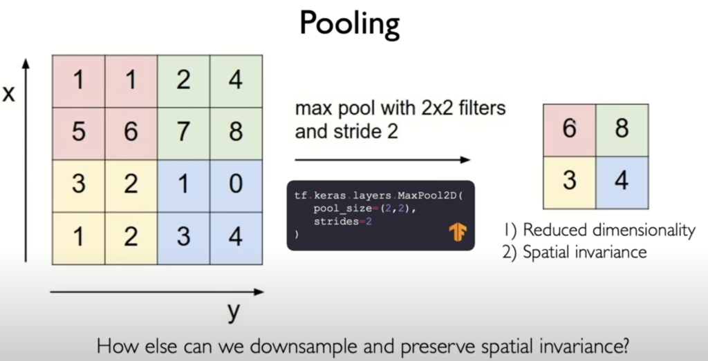
- Pooling:
- Purpose: Reduces the dimensionality of the feature maps to manage computational complexity and prevent overfitting.
- Common Technique: Max pooling.
- Function: Divides the input feature map into smaller regions (e.g., 2×2 grids) and outputs the maximum value from each region, effectively reducing the size of the feature map by a factor of two. This retains the most significant features while reducing data volume.
- Alternative Methods: Average pooling, which outputs the average value of each region instead of the maximum, among other methods.
Full Convolutional Layer:
- Composition: Convolution followed by non-linearity (e.g., ReLU) and pooling.
- Purpose: Each layer extracts progressively more complex features, building hierarchical representations from low-level edges to high-level object parts.
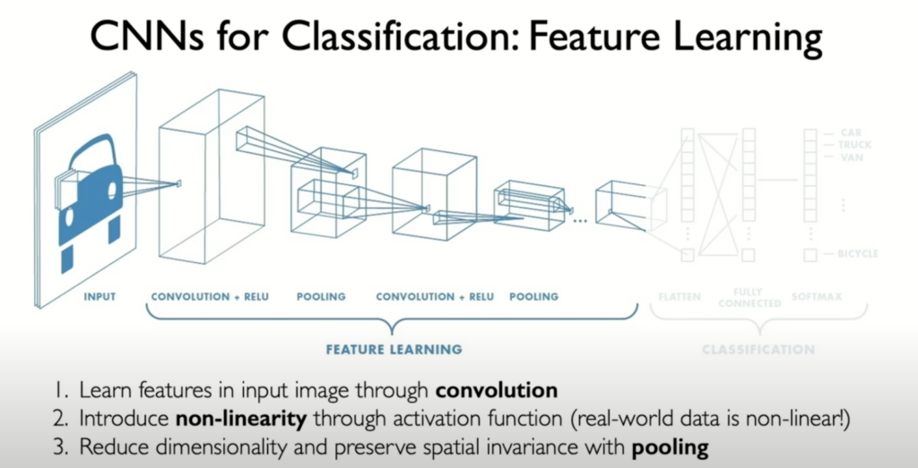
CNN Structure for Image Classification:
- Feature Extraction Head: Composed of multiple convolutional layers to extract relevant features from the input image.
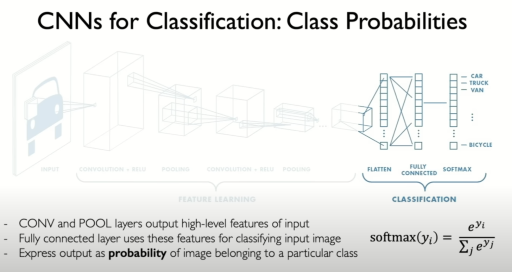
- Classification Head: After feature extraction, the features are fed into fully connected layers to perform classification. This step often uses a softmax function to produce a probability distribution over classes.
Overall Workflow:
- Input image is processed through convolutional layers to extract features.
- Features are pooled to reduce dimensionality while retaining important information.
- Extracted features are fed into fully connected layers for classification.
- The softmax function ensures the output probabilities sum to one, suitable for categorization tasks.
This process enables CNNs to efficiently learn and classify visual patterns by leveraging hierarchical feature extraction and dimensionality reduction.
Convolutional Neural Networks Architecture: A Two-Part Symphony
A CNN for image classification can be viewed as a two-part system:
- Feature Extraction: This part consists of stacked convolutional layers interspersed with non-linearity and pooling layers. It learns hierarchical representations of the image, going from simple edges and textures in early layers to complex object parts in later layers.
- Classification: The final layers of the network are typically fully connected, taking the learned features as input and outputting a probability distribution over the possible classes.
Beyond Classification: The Versatility of CNN
The real beauty of CNNs lies in their modularity. By swapping out the classification head with different types of layers, we can adapt CNNs for a wide range of computer vision tasks:
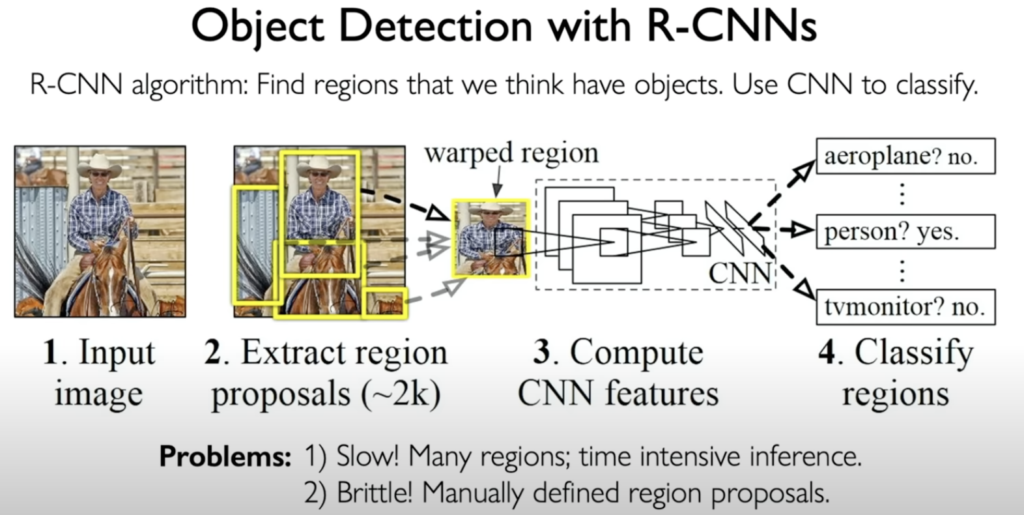
- Object Detection: Instead of just classifying the entire image, object detection involves identifying the locations of multiple objects within an image and drawing bounding boxes around them. Techniques like Faster R-CNN that use region proposal networks to efficiently identify potential object locations.
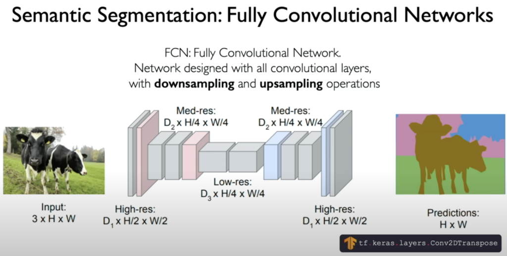
- Semantic Segmentation: This task takes object detection a step further by classifying every single pixel in the image. The output is a segmented image where each pixel is labeled with its corresponding class (e.g., road, sky, car).
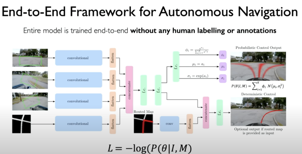
- Self-Driving Cars: CNNs are crucial for enabling autonomous driving. They can process camera images to detect lanes, traffic signs, pedestrians, and other vehicles, providing essential information for navigation. The lecture showcases an impressive example of a CNN-powered car navigating a new environment without any prior knowledge of the route.
Conclusion
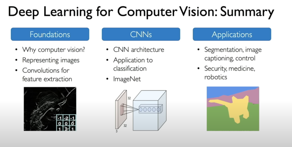
In this blog we learned about CNNs, demystifying their inner workings and showcasing their impressive capabilities in solving various computer vision tasks. From medical diagnosis to self-driving cars, CNNs are revolutionizing numerous fields. As research progresses, we can expect even more innovative applications of these powerful deep learning models in the future.
For a complete video check this video or visit the website