Introduction
Intelligence: The ability to process information and use it for future decision-making.
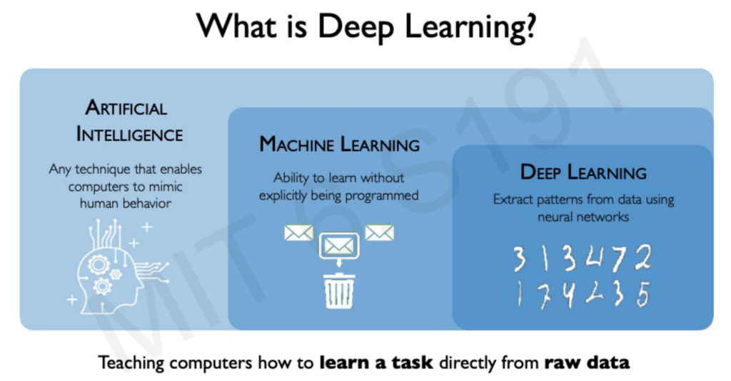
Artificial Intelligence (AI): Empowering computers with the ability to process information and make decisions.
Machine Learning (ML): A subset of AI focused on teaching computers to learn from data.
Deep Learning (DL): A subset of ML utilizing neural networks to process raw data and inform decisions.
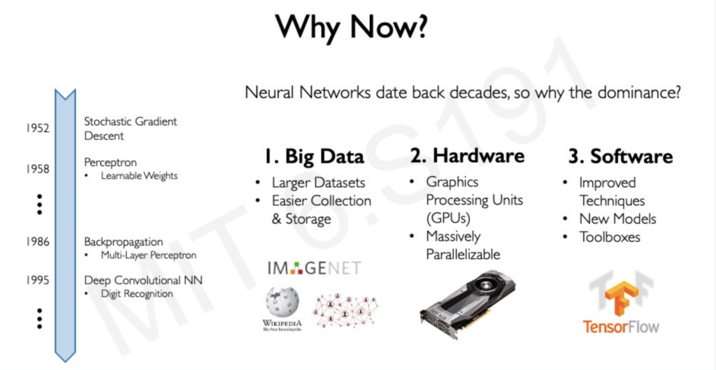
Why Deep Learning Now?
The recent surge in deep learning’s capabilities can be attributed to three key factors:
- Data Explosion: Deep learning models thrive on data, and we’re currently experiencing an unprecedented level of data generation.
- Hardware Advancements: GPUs offer the parallel processing power necessary for deep learning algorithms.
- Open-Source Software: Tools like TensorFlow and PyTorch have streamlined the development and deployment of deep learning models.
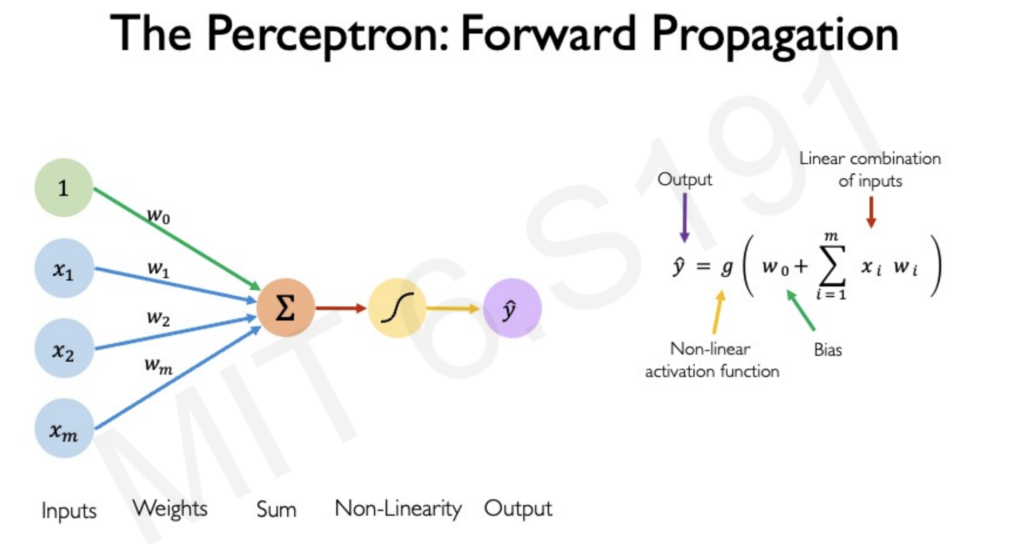
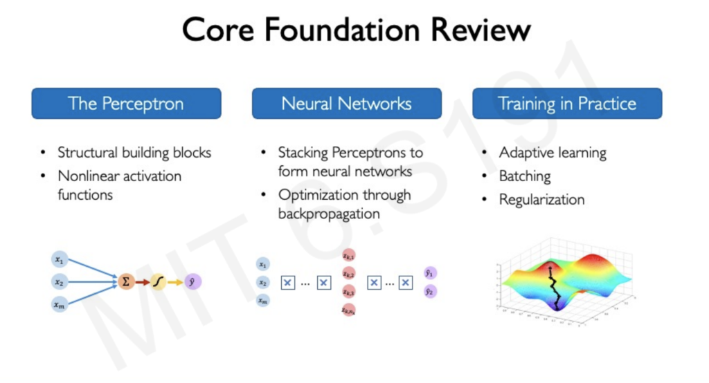
The Perceptron: A Neural Network Building Block
The fundamental building block of a neural network is the perceptron, a single neuron that processes information through three steps:
- Dot Product: Multiplying inputs with corresponding weights.
- Bias Addition: Adding a bias term to shift the activation function.
- Nonlinear Activation: Passing the result through a nonlinear function like sigmoid or ReLU.
Common Activation Functions
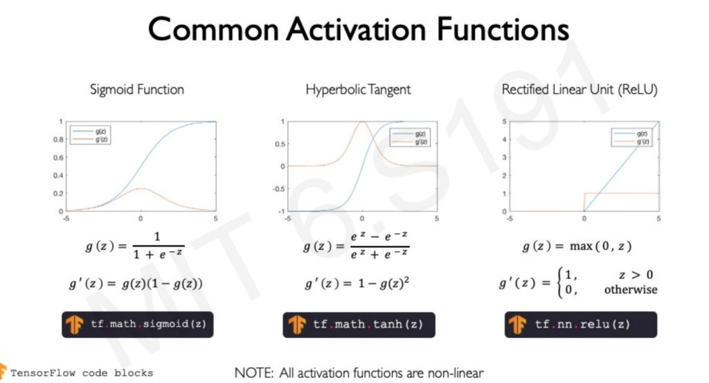
- Sigmoid: This function squashes any input value to a range between 0 and 1, making it suitable for modeling probabilities. However, it suffers from the vanishing gradient problem, where gradients become very small during backpropagation, hindering learning in early layers of deep networks.
- ReLU (Rectified Linear Unit): This simple function outputs the input directly if it’s positive; otherwise, it outputs zero. ReLU is computationally efficient and doesn’t suffer from the vanishing gradient problem as much as sigmoid. However, it can suffer from the “dying ReLU” problem, where neurons get stuck in a state where they always output zero.
- Tanh (Hyperbolic Tangent): Tanh is similar to sigmoid but outputs values between -1 and 1. It’s often preferred over sigmoid as it centers the data around zero, which can aid in learning. However, it still suffers from the vanishing gradient problem.
Why Nonlinearity is Essential
- Real-World Data is Nonlinear: Real-world phenomena are rarely linear. Imagine trying to classify images of cats and dogs – a linear function wouldn’t be able to capture the complex patterns and features that distinguish the two animals. Nonlinear activation functions allow neural networks to learn these intricate relationships within the data.
- Expressive Power: Nonlinearity enables neural networks to learn more complex functions. Stacking multiple linear layers would still result in a linear model, limiting the network’s ability to handle intricate patterns. Nonlinear activations provide the necessary expressiveness for tackling challenging tasks.
- Decision Boundaries: Nonlinear activations enable the creation of non-linear decision boundaries, which are crucial for classification tasks. For example, a linear function could only separate data points with a straight line, whereas a nonlinear function can learn curves and complex shapes to accurately separate different classes.
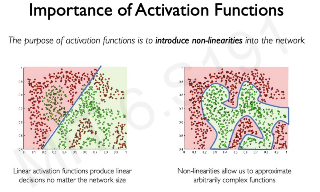
In essence, nonlinear activation functions are the key to unlocking the power of deep learning. They allow neural networks to learn the complex representations and relationships present in real-world data, enabling them to perform a wide range of tasks with remarkable accuracy.
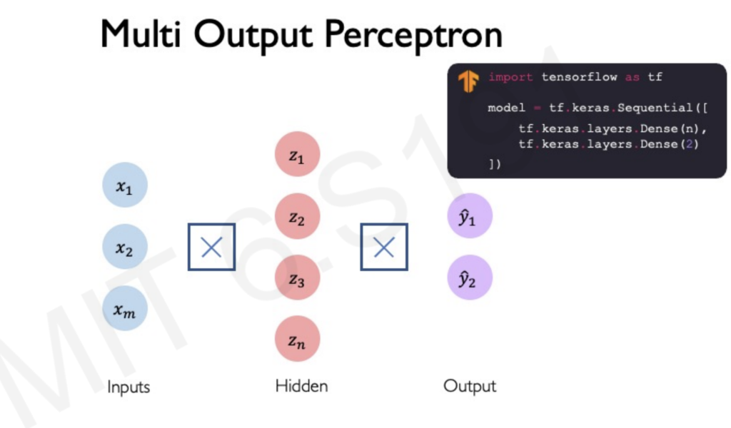
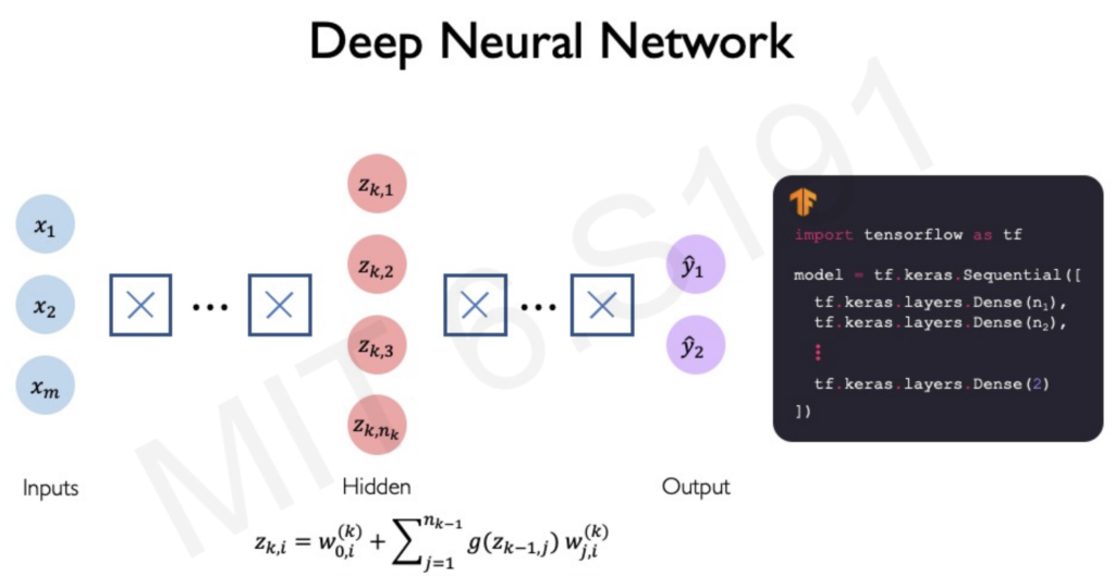
Building Neural Networks
Multiple perceptrons connected in layers form a neural network. Deep learning involves stacking these layers, creating a hierarchy that allows for complex data processing.
Challenges in Training Neural Networks
Training neural networks comes with challenges:
- Computational Cost: Backpropagation, the algorithm for computing gradients, can be computationally expensive.
- Local Minima: Gradient descent can get stuck in local minima instead of reaching the global minimum.
- Overfitting: Models may learn the training data too well and fail to generalize to new data.
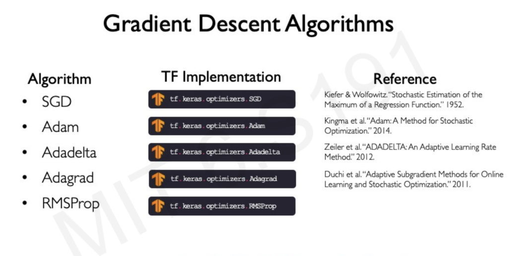
Techniques like stochastic gradient descent (SGD), adaptive learning rates, dropout, and early stopping help address these challenges.
Gradient Descent and Stochastic Gradient Descent: Navigating the Loss Landscape
The journey of training a neural network revolves around finding the optimal set of weights that minimize the error between its predictions and the actual target values. This is where gradient descent comes into play, acting as a guide through the complex terrain of the loss landscape.
Understanding the Loss Landscape:
Imagine a mountainous landscape where each point represents a specific configuration of weights for the neural network, and the height at each point signifies the corresponding loss (error) value. Our goal is to reach the lowest point in this landscape, representing the set of weights that yield the minimum loss.
Gradient Descent: Taking Small Steps Downward:
Gradient descent is an iterative optimization algorithm that helps us navigate this loss landscape. It works by taking small steps in the direction of the steepest descent, gradually approaching the minimum loss. Here’s how it operates:
- Initialization: We start at a random point in the loss landscape (a random set of weights).
- Gradient Calculation: We compute the gradient at our current location, which indicates the direction of the steepest ascent.
- Step in the Opposite Direction: We take a small step in the opposite direction of the gradient, effectively moving towards a lower point in the landscape.
- Repeat: We iterate steps 2 and 3 until we reach a point where further steps no longer significantly decrease the loss.
The Learning Rate: Controlling the Step Size:
The size of the steps taken in gradient descent is determined by the learning rate. Setting the learning rate is crucial:
- Too small: The model may take too long to converge or get stuck in local minima.
- Too large: The model may overshoot the minimum and diverge.
Stochastic Gradient Descent: Efficiency through Approximation:
Traditional gradient descent calculates the gradient using the entire training dataset, which can be computationally expensive for large datasets. Stochastic Gradient Descent (SGD) offers a more efficient approach by approximating the gradient using a single data point or a small batch of data points (mini-batch).
This introduces some noise into the process but allows for faster iterations and often leads to quicker convergence. The trade-off between accuracy and efficiency is a key consideration when choosing between gradient descent and SGD.
Key Takeaways:
- Gradient descent and SGD are optimization algorithms that guide the training process of neural networks by iteratively adjusting weights to minimize the loss.
- The learning rate controls the step size in gradient descent and needs to be carefully tuned for optimal performance.
- SGD offers computational efficiency by approximating the gradient using smaller batches of data, but at the cost of introducing noise.
In essence, gradient descent and its variants are the driving force behind training neural networks, allowing them to learn from data and achieve remarkable results in various AI applications.
Understanding Overfitting
Overfitting results in models that perform exceptionally well on the training data but fail to generalize to new, unseen examples. Imagine a student who memorizes every answer in a textbook but struggles to apply that knowledge to real-world problems. That’s essentially what happens with an overfitted model.
Regularization to the Rescue
To combat overfitting, we turn to regularization techniques. These techniques aim to discourage the model from learning the idiosyncrasies of the training data and instead encourage it to learn more generalizable patterns.
Two Key Regularization Techniques:
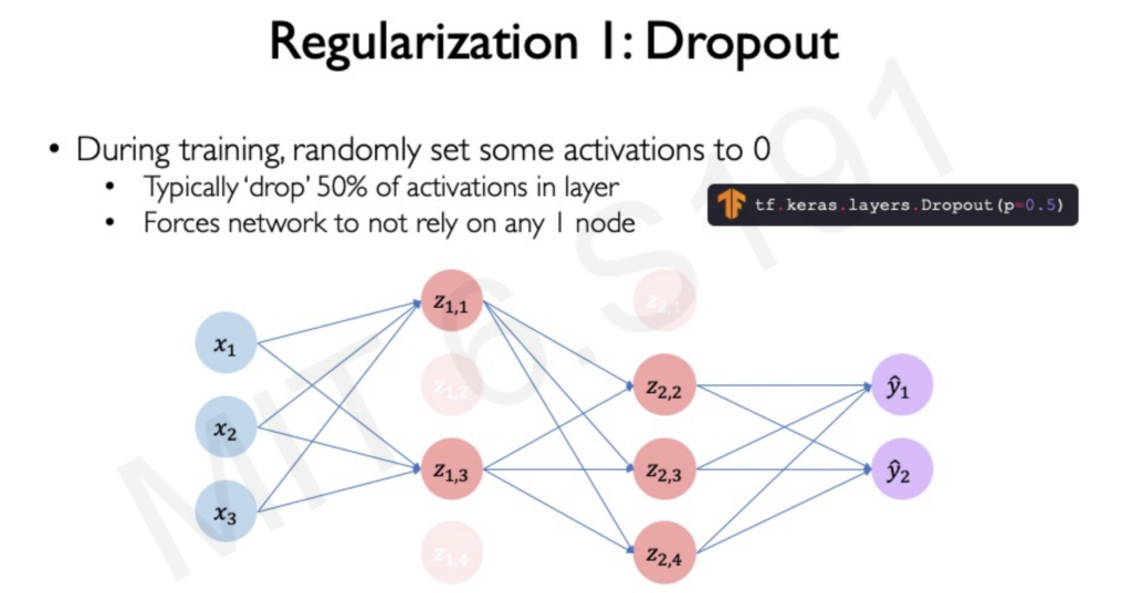
- Dropout: During training, dropout randomly sets a portion of neuron activations to zero. This forces the network to learn redundant representations, as it cannot rely on the presence of specific neurons. By preventing reliance on any single feature, dropout improves the model’s ability to generalize.
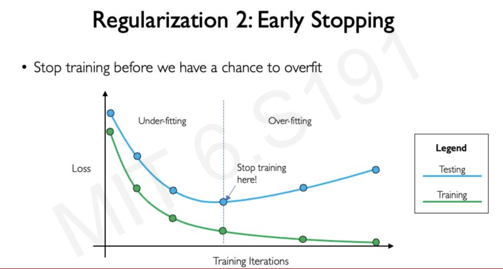
- Early Stopping: This technique involves monitoring the model’s performance on both the training data and a separate validation set during training. When the validation loss starts to increase, it indicates that the model is beginning to overfit. Early stopping simply halts the training process at this point, preventing further memorization of the training data and preserving the model’s ability to generalize.
Why Regularization Matters
Regularization plays a crucial role in ensuring that deep learning models are not just good at memorizing training data but can effectively handle real-world scenarios and new data points. By preventing overfitting, regularization techniques help us build robust and reliable AI systems.
Review
Video
For complete course check this link