What are vector databases?
A Vector Database is a type of database that stores information in a structured way using vectors. Now, what are vectors? Think of them as mathematical representations of data that capture its meaning and context.
Let’s say you have a photo of a cat. Instead of just storing the image file, a Vector Database will convert this photo into a vector, which is essentially a set of numbers that represent various features of the cat, like its color, shape, and size. This vector will contain information about the cat in a way that a computer can understand.
Now, the cool thing about vector databases is that they allow you to search for similar items easily. For instance, if you upload a photo of a dog, the database can quickly find other photos with similar features to that dog by comparing their vectors. This is like when you search for similar images on your smartphone—except it’s done using mathematical calculations rather than just looking for file names or tags.
So, in simple terms, a Vector Database helps organize and search for different types of data by converting them into mathematical representations called vectors, making it easier to find similar items or information.
Check Understanding Embeddings: https://learncodecamp.net/embeddings/
Vector databases are specialized databases tailored for high-dimensional data points represented as vectors, offering efficient storage and retrieval capabilities. They excel at performing nearest-neighbor searches, swiftly retrieving data points closest to a given point in multi-dimensional space.
Key techniques employed in vector databases
- k-Nearest Neighbor (k-NN) Index: This technique enables rapid identification of the k nearest neighbors of a given vector. It aids in efficiently narrowing down the search space, improving retrieval speed.
- Hierarchical Navigable Small World (HNSW): HNSW algorithm efficiently organizes data points to facilitate faster nearest-neighbor searches. It constructs a hierarchical graph structure that optimizes the search process.
In summary, vector databases leverage advanced methods such as k-NN indexes and algorithms like HNSW to ensure efficient storage and retrieval of high-dimensional vectors, enabling rapid lookup of nearest neighbors in multi-dimensional spaces.
# Function to find K Nearest Neighbors
def find_k_nearest_neighbors(query_vector, vectors, k=5, threshold=0.8):
    nearest_neighbors = []
    for vector in vectors:
        similarity = cosine_similarity(query_vector, vector)
        if similarity >= threshold:
            nearest_neighbors.append((vector, similarity))
    nearest_neighbors.sort(key=lambda x: x[1], reverse=True)
    return nearest_neighbors[:k]
Simple pseudocode for finding k nearest neighbors, query_vector is the embedding vector of the search term, and k is the number of the items to retrieve, threshold is minimum match %
The brute force of a kNN search is computationally very expensive – and depending on the size of your database, a single query could take anything from several seconds to even mins.
Number of computations = Number of dimensions × Vector size
Given:
- Number of dimensions (d) = 1536
- Vector size (n) = 1 million = 1×10^6
Number of computations=1536×1×10^6 = 1.536×10^9 approximately 1.536 billion
it would take approximately 1.536 seconds to perform all the computations needed for your kNN search on a system capable of performing 1 billion computations per second.
Let’s explore Approximate Nearest Neighbors Algorithms.
Approximate Nearest Neighbors Search (K-ANNS)
This is used to efficiently find approximate nearest neighbors for a given query point in a large dataset. It’s particularly useful when dealing with high-dimensional data where traditional exact nearest neighbor search methods become computationally expensive.
The quality of an inexact search (the recall) is defined as the ratio between the number of found true nearest neighbors and K
To elaborate:
- True Nearest Neighbors: These are the actual nearest neighbors of the query point in the dataset, determined by some distance metric. For example, if we’re searching for the 5 nearest neighbors (K=5) of a given point, the true nearest neighbors are those 5 points in the dataset that are closest to the query point.
- Found Nearest Neighbors: These are the points that the approximate search algorithm returns as the nearest neighbors of the query point. Due to the approximate nature of the search, they may not be exactly the same as the true nearest neighbors.
- Recall: The recall of the search is then defined as the ratio of the number of found true nearest neighbors to the total number of nearest neighbors desired (K). It’s calculated using the formula:
Recall = (Number of Found True Nearest Neighbors) / K
For example, if a search algorithm returns 3 out of the 5 true nearest neighbors for a query with K=5, the recall would be 3/5, or 0.6. This means that the algorithm successfully retrieved 60% of the true nearest neighbors.
High recall is desirable in many applications because it indicates that the algorithm is effectively capturing the most relevant points in the dataset.
Examples of ANN algorithms
Examples of ANN methods are:
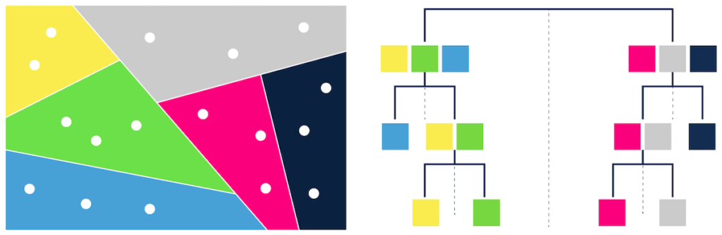
- trees – e.g. ANNOY (Figure 1),
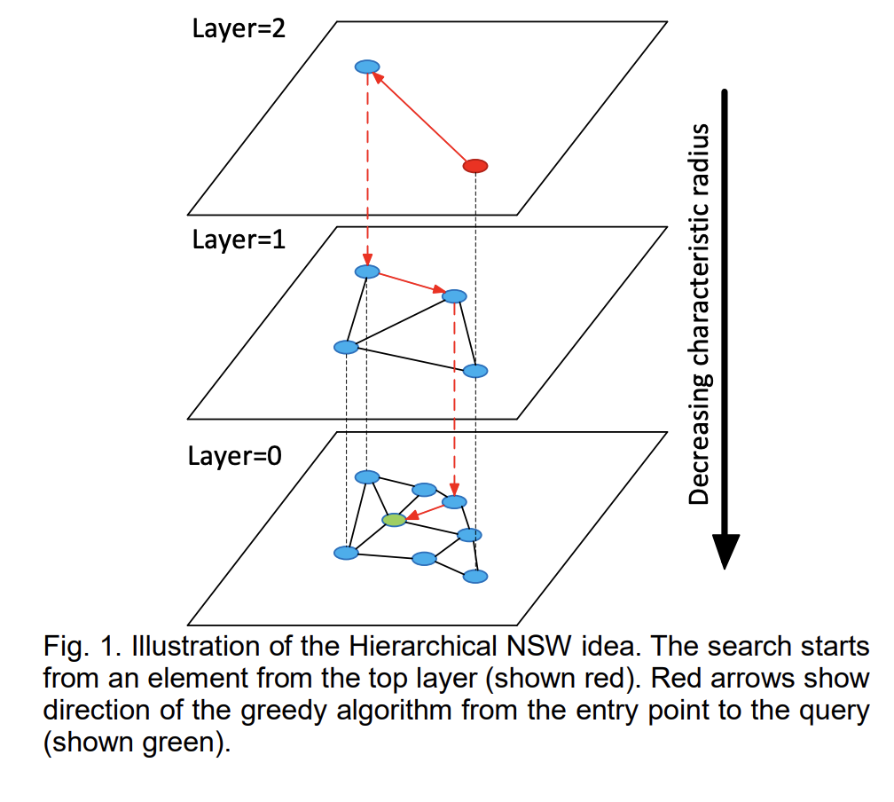
- proximity graphs – e.g. HNSW (Figure 2),
- clustering – e.g. FAISS,
- hashing – e.g. LSH,
- vector compression – e.g. PQ or SCANN.
Annoy is used at Spotify for music recommendations. Redis Search supports FLAT – Brute-force index and HNSW
HNSW
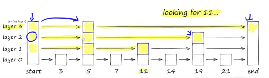
Probabilistic Skip List: A skip list is a data structure that allows for fast search, insertion, and deletion operations in a sorted list. It achieves this by adding multiple layers of pointers, allowing for “skipping” over some elements during traversal. In HNSW, the probabilistic skip list is used to organize the data points within each layer of the hierarchical structure.
The “Navigable Small World” (NSW) part of Hierarchical Navigable Small World (HNSW) refers to a graph structure designed to maintain both local connectivity and global exploration capabilities. Let’s break down the NSW component:
- Navigability: NSW aims to create a graph structure where each data point (or node) is connected to its neighbors in a way that facilitates efficient navigation through the dataset. This means that similar points are likely to be connected, allowing for quick traversal between them.
- Small World Property: The small-world property refers to the idea that even though the graph may be large and sparsely connected, it’s still possible to navigate from one point to another through a relatively small number of connections. This property is essential for efficient search and exploration in large datasets.
- Connection Strategy: In NSW, connections between points are established based on their proximity in the data space. Typically, points that are closer together in the data space are more likely to be connected. However, NSW also incorporates randomness into the connection strategy to balance local connectivity with global exploration.
- Efficient Search: By creating a graph structure with the small-world property, NSW enables efficient search for nearest neighbors. During the search process, the algorithm can navigate through the graph using a combination of local connections to quickly find nearby points and occasional long-range connections to explore distant regions of the dataset.
Summary
- Vector databases rely on Machine Learning models to generate vector embeddings for all data objects.
- Vector embeddings represent the meaning and context of data, enabling efficient analysis and retrieval.
- Vector databases provide rapid query capabilities due to Approximate Nearest Neighbors (ANN) algorithms.
- ANN algorithms sacrifice some accuracy in exchange for significant performance improvements.